Z-score Table

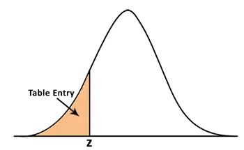
This Negative Z Table can help you find the values that are left of the mean. Table entries for Z define the area under the standard normal curve to the left of the Z. The negative score represents the corresponding values that are less than the mean.

Z	0	0.01	0.02	0.03	0.04	0.05	0.06	0.07	0.08	0.09
-3.9	0.00005	0.00005	0.00004	0.00004	0.00004	0.00004	0.00004	0.00004	0.00003	0.00003
-3.8	0.00007	0.00007	0.00007	0.00006	0.00006	0.00006	0.00006	0.00005	0.00005	0.00005
-3.7	0.00011	0.0001	0.0001	0.0001	0.00009	0.00009	0.00008	0.00008	0.00008	0.00008
-3.6	0.00016	0.00015	0.00015	0.00014	0.00014	0.00013	0.00013	0.00012	0.00012	0.00011
-3.5	0.00023	0.00022	0.00022	0.00021	0.0002	0.00019	0.00019	0.00018	0.00017	0.00017
-3.4	0.00034	0.00032	0.00031	0.0003	0.00029	0.00028	0.00027	0.00026	0.00025	0.00024
-3.3	0.00048	0.00047	0.00045	0.00043	0.00042	0.0004	0.00039	0.00038	0.00036	0.00035
-3.2	0.00069	0.00066	0.00064	0.00062	0.0006	0.00058	0.00056	0.00054	0.00052	0.0005
-3.1	0.00097	0.00094	0.0009	0.00087	0.00084	0.00082	0.00079	0.00076	0.00074	0.00071
-3	0.00135	0.00131	0.00126	0.00122	0.00118	0.00114	0.00111	0.00107	0.00104	0.001
-2.9	0.00187	0.00181	0.00175	0.00169	0.00164	0.00159	0.00154	0.00149	0.00144	0.00139
-2.8	0.00256	0.00248	0.0024	0.00233	0.00226	0.00219	0.00212	0.00205	0.00199	0.00193
-2.7	0.00347	0.00336	0.00326	0.00317	0.00307	0.00298	0.00289	0.0028	0.00272	0.00264
-2.6	0.00466	0.00453	0.0044	0.00427	0.00415	0.00402	0.00391	0.00379	0.00368	0.00357
-2.5	0.00621	0.00604	0.00587	0.0057	0.00554	0.00539	0.00523	0.00508	0.00494	0.0048
-2.4	0.0082	0.00798	0.00776	0.00755	0.00734	0.00714	0.00695	0.00676	0.00657	0.00639
-2.3	0.01072	0.01044	0.01017	0.0099	0.00964	0.00939	0.00914	0.00889	0.00866	0.00842
-2.2	0.0139	0.01355	0.01321	0.01287	0.01255	0.01222	0.01191	0.0116	0.0113	0.01101
-2.1	0.01786	0.01743	0.017	0.01659	0.01618	0.01578	0.01539	0.015	0.01463	0.01426
-2	0.02275	0.02222	0.02169	0.02118	0.02068	0.02018	0.0197	0.01923	0.01876	0.01831
-1.9	0.02872	0.02807	0.02743	0.0268	0.02619	0.02559	0.025	0.02442	0.02385	0.0233
-1.8	0.03593	0.03515	0.03438	0.03362	0.03288	0.03216	0.03144	0.03074	0.03005	0.02938
-1.7	0.04457	0.04363	0.04272	0.04182	0.04093	0.04006	0.0392	0.03836	0.03754	0.03673
-1.6	0.0548	0.0537	0.05262	0.05155	0.0505	0.04947	0.04846	0.04746	0.04648	0.04551
-1.5	0.06681	0.06552	0.06426	0.06301	0.06178	0.06057	0.05938	0.05821	0.05705	0.05592
-1.4	0.08076	0.07927	0.0778	0.07636	0.07493	0.07353	0.07215	0.07078	0.06944	0.06811
-1.3	0.0968	0.0951	0.09342	0.09176	0.09012	0.08851	0.08691	0.08534	0.08379	0.08226
-1.2	0.11507	0.11314	0.11123	0.10935	0.10749	0.10565	0.10383	0.10204	0.10027	0.09853
-1.1	0.13567	0.1335	0.13136	0.12924	0.12714	0.12507	0.12302	0.121	0.119	0.11702
-1	0.15866	0.15625	0.15386	0.15151	0.14917	0.14686	0.14457	0.14231	0.14007	0.13786
-0.9	0.18406	0.18141	0.17879	0.17619	0.17361	0.17106	0.16853	0.16602	0.16354	0.16109
-0.8	0.21186	0.20897	0.20611	0.20327	0.20045	0.19766	0.19489	0.19215	0.18943	0.18673
-0.7	0.24196	0.23885	0.23576	0.2327	0.22965	0.22663	0.22363	0.22065	0.2177	0.21476
-0.6	0.27425	0.27093	0.26763	0.26435	0.26109	0.25785	0.25463	0.25143	0.24825	0.2451
-0.5	0.30854	0.30503	0.30153	0.29806	0.2946	0.29116	0.28774	0.28434	0.28096	0.2776
-0.4	0.34458	0.3409	0.33724	0.3336	0.32997	0.32636	0.32276	0.31918	0.31561	0.31207
-0.3	0.38209	0.37828	0.37448	0.3707	0.36693	0.36317	0.35942	0.35569	0.35197	0.34827
-0.2	0.42074	0.41683	0.41294	0.40905	0.40517	0.40129	0.39743	0.39358	0.38974	0.38591
-0.1	0.46017	0.4562	0.45224	0.44828	0.44433	0.44038	0.43644	0.43251	0.42858	0.42465
0	0.5	0.49601	0.49202	0.48803	0.48405	0.48006	0.47608	0.4721	0.46812	0.46414

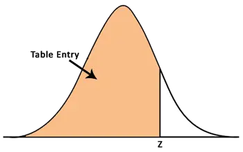
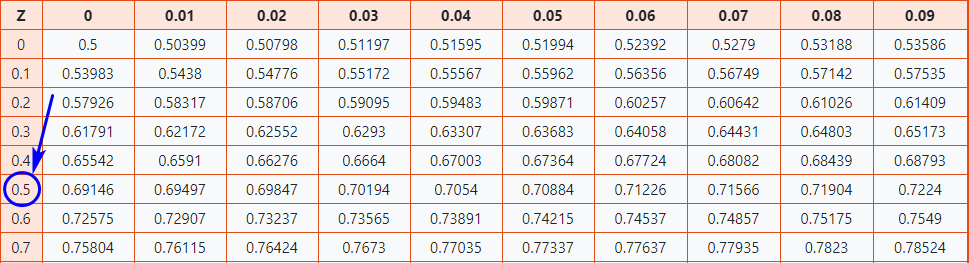
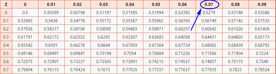
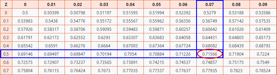
The positive Z-score table is used to find the values that are right from the mean. The table entries for Z define the area under the standard normal curve to the left of the Z. Positive Z-score represents the corresponding values greater than the mean.

Z	0	0.01	0.02	0.03	0.04	0.05	0.06	0.07	0.08	0.09
0	0.5	0.50399	0.50798	0.51197	0.51595	0.51994	0.52392	0.5279	0.53188	0.53586
0.1	0.53983	0.5438	0.54776	0.55172	0.55567	0.55962	0.56356	0.56749	0.57142	0.57535
0.2	0.57926	0.58317	0.58706	0.59095	0.59483	0.59871	0.60257	0.60642	0.61026	0.61409
0.3	0.61791	0.62172	0.62552	0.6293	0.63307	0.63683	0.64058	0.64431	0.64803	0.65173
0.4	0.65542	0.6591	0.66276	0.6664	0.67003	0.67364	0.67724	0.68082	0.68439	0.68793
0.5	0.69146	0.69497	0.69847	0.70194	0.7054	0.70884	0.71226	0.71566	0.71904	0.7224
0.6	0.72575	0.72907	0.73237	0.73565	0.73891	0.74215	0.74537	0.74857	0.75175	0.7549
0.7	0.75804	0.76115	0.76424	0.7673	0.77035	0.77337	0.77637	0.77935	0.7823	0.78524
0.8	0.78814	0.79103	0.79389	0.79673	0.79955	0.80234	0.80511	0.80785	0.81057	0.81327
0.9	0.81594	0.81859	0.82121	0.82381	0.82639	0.82894	0.83147	0.83398	0.83646	0.83891
1	0.84134	0.84375	0.84614	0.84849	0.85083	0.85314	0.85543	0.85769	0.85993	0.86214
1.1	0.86433	0.8665	0.86864	0.87076	0.87286	0.87493	0.87698	0.879	0.881	0.88298
1.2	0.88493	0.88686	0.88877	0.89065	0.89251	0.89435	0.89617	0.89796	0.89973	0.90147
1.3	0.9032	0.9049	0.90658	0.90824	0.90988	0.91149	0.91309	0.91466	0.91621	0.91774
1.4	0.91924	0.92073	0.9222	0.92364	0.92507	0.92647	0.92785	0.92922	0.93056	0.93189
1.5	0.93319	0.93448	0.93574	0.93699	0.93822	0.93943	0.94062	0.94179	0.94295	0.94408
1.6	0.9452	0.9463	0.94738	0.94845	0.9495	0.95053	0.95154	0.95254	0.95352	0.95449
1.7	0.95543	0.95637	0.95728	0.95818	0.95907	0.95994	0.9608	0.96164	0.96246	0.96327
1.8	0.96407	0.96485	0.96562	0.96638	0.96712	0.96784	0.96856	0.96926	0.96995	0.97062
1.9	0.97128	0.97193	0.97257	0.9732	0.97381	0.97441	0.975	0.97558	0.97615	0.9767
2	0.97725	0.97778	0.97831	0.97882	0.97932	0.97982	0.9803	0.98077	0.98124	0.98169
2.1	0.98214	0.98257	0.983	0.98341	0.98382	0.98422	0.98461	0.985	0.98537	0.98574
2.2	0.9861	0.98645	0.98679	0.98713	0.98745	0.98778	0.98809	0.9884	0.9887	0.98899
2.3	0.98928	0.98956	0.98983	0.9901	0.99036	0.99061	0.99086	0.99111	0.99134	0.99158
2.4	0.9918	0.99202	0.99224	0.99245	0.99266	0.99286	0.99305	0.99324	0.99343	0.99361
2.5	0.99379	0.99396	0.99413	0.9943	0.99446	0.99461	0.99477	0.99492	0.99506	0.9952
2.6	0.99534	0.99547	0.9956	0.99573	0.99585	0.99598	0.99609	0.99621	0.99632	0.99643
2.7	0.99653	0.99664	0.99674	0.99683	0.99693	0.99702	0.99711	0.9972	0.99728	0.99736
2.8	0.99744	0.99752	0.9976	0.99767	0.99774	0.99781	0.99788	0.99795	0.99801	0.99807
2.9	0.99813	0.99819	0.99825	0.99831	0.99836	0.99841	0.99846	0.99851	0.99856	0.99861
3	0.99865	0.99869	0.99874	0.99878	0.99882	0.99886	0.99889	0.99893	0.99896	0.999
3.1	0.99903	0.99906	0.9991	0.99913	0.99916	0.99918	0.99921	0.99924	0.99926	0.99929
3.2	0.99931	0.99934	0.99936	0.99938	0.9994	0.99942	0.99944	0.99946	0.99948	0.9995
3.3	0.99952	0.99953	0.99955	0.99957	0.99958	0.9996	0.99961	0.99962	0.99964	0.99965
3.4	0.99966	0.99968	0.99969	0.9997	0.99971	0.99972	0.99973	0.99974	0.99975	0.99976
3.5	0.99977	0.99978	0.99978	0.99979	0.9998	0.99981	0.99981	0.99982	0.99983	0.99983
3.6	0.99984	0.99985	0.99985	0.99986	0.99986	0.99987	0.99987	0.99988	0.99988	0.99989
3.7	0.99989	0.9999	0.9999	0.9999	0.99991	0.99991	0.99992	0.99992	0.99992	0.99992
3.8	0.99993	0.99993	0.99993	0.99994	0.99994	0.99994	0.99994	0.99995	0.99995	0.99995
3.9	0.99995	0.99995	0.99996	0.99996	0.99996	0.99996	0.99996	0.99996	0.99997	0.99997

Standard Normal Distribution Table PDF →

Z-score Table

How to Calculate Z-score?

How to Read the Z Table?

1. Check the first two digits on Y-axis

2. Check the second decimal number on X-axis

3. Join the X and Y axis

4. Convert the resultant value into a percentage